We say «there is a 30% chance of rain», «the coin has a one-half probability of landing heads», «the server probably went down because of an update». We use the same word for very different things. Before doing any calculation it is worth clarifying what we mean, because the different interpretations lead to different ways of reasoning about data, even though they share the same mathematical rules.
Three ways to read a number between 0 and 1
Classical probability
This is the oldest definition, born from the study of games of chance: the probability of an event is the ratio of favourable cases to possible cases, provided all cases are equally possible. Rolling a fair die, the probability of getting an even number is 3/6 = 1/2.
The limitation is obvious: it only works when we can list symmetric outcomes. It tells us nothing about a loaded die, the lifetime of a hard disk or the probability that an email is spam. Moreover, the condition «equally possible» risks being circular, because it already presupposes an idea of probability.
Frequentist probability
Here probability is the relative frequency with which an event occurs in a long series of trials repeated under the same conditions. If we toss a coin ten thousand times and get heads 5,030 times, we estimate the probability of heads at around 0.503.
This reading underpins classical statistics: hypothesis tests, confidence intervals, p-values. Its strength is that it is anchored to observable data, but it struggles with one-off events: what does it mean to speak of the frequency with which «this project will finish on time»?
Subjective (or Bayesian) probability
In this interpretation probability measures a rational person's degree of belief in a statement, given what they know. Two people with different information can assign different probabilities to the same event without either being wrong. Belief is not arbitrary, though: it must obey the rules of the calculus and be updated when new data arrive, through Bayes' theorem.
It is the natural approach for single events and for combining prior information with new observations, as spam filters and many diagnostic systems do.
The shared rules: Kolmogorov's axioms
In 1933 the Russian mathematician Andrey Kolmogorov proposed an axiomatic formulation that does not depend on interpretation. It needs three ingredients:
- a sample space Ω, the set of all possible outcomes (for a die: {1, 2, 3, 4, 5, 6});
- a family of events, that is, subsets of Ω (for example «an even number comes up» = {2, 4, 6});
- a function P that assigns a number to each event.
There are three axioms:
- Non-negativity: P(A) ≥ 0 for every event A.
- Normalisation: P(Ω) = 1, meaning that something certainly happens.
- Additivity: if A and B are mutually exclusive (they cannot happen together), P(A or B) = P(A) + P(B). The full version extends the rule to infinite sequences of pairwise exclusive events.
Everything else can be proved from here.
Useful consequences in practice
Complementary event
Since A and «not A» are mutually exclusive and together cover Ω, we have P(not A) = 1 − P(A). It is a very powerful trick: it is often easier to compute the probability that something does not happen. The probability of getting at least one six in four rolls of a die is 1 − (5/6)⁴ ≈ 0.518, far quicker to obtain than by adding up all the cases.
Union of compatible events
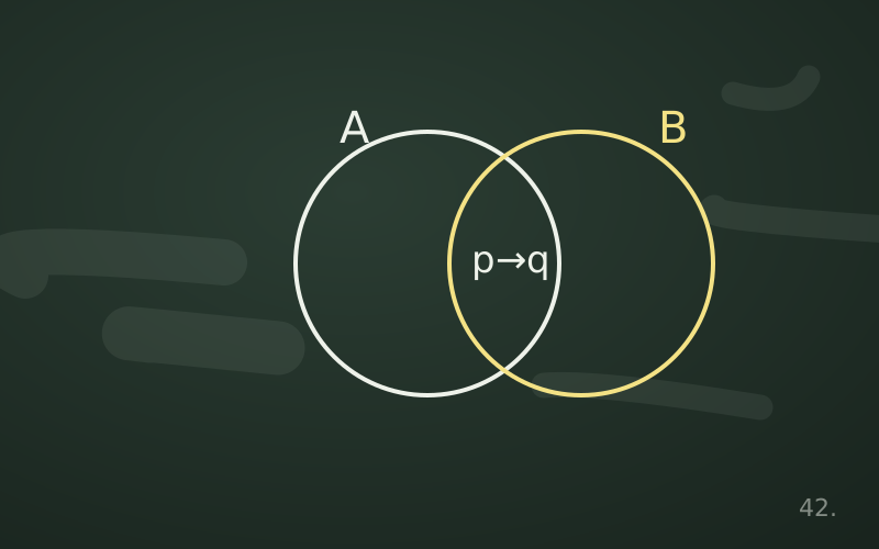
If A and B can happen together, adding them counts the intersection twice. The correct rule is:
P(A or B) = P(A) + P(B) − P(A and B)
Example with a 52-card deck: the probability of drawing a heart or a face card (J, Q, K) is 13/52 + 12/52 − 3/52 = 22/52, because the three face cards of hearts must be counted only once.
Monotonicity and limits
If A implies B, then P(A) ≤ P(B). It seems obvious, yet intuitive reasoning violates it often: we judge a detailed story («the attack started with a phishing email and exploited a reused password») more probable than one of its parts («the attack exploited a reused password»). Adding details makes a story more convincing, but never more probable.
Why interpretation matters
The rules are identical for everyone, but the interpretation changes which questions are legitimate. A frequentist does not assign a probability to a hypothesis («the drug works»): the hypothesis is either true or false, and probability concerns the data we might observe. A Bayesian, by contrast, can say «given the data, the probability that the drug works is 0.9». Many misreadings of p-values arise precisely from confusing the two perspectives.
In my work with logs and incidents I often use both: historical frequencies provide a starting point, and Bayesian reasoning helps update it when new clues emerge.
| Interpretation | What it measures | Where it works best |
|---|---|---|
| Classical | Favourable cases over possible cases | Games with symmetric outcomes |
| Frequentist | Long-run frequency | Repeatable experiments, quality control |
| Subjective | Coherent degree of belief | One-off events, updating with new data |
In short
- Probability has at least three readings: classical, frequentist and subjective.
- Kolmogorov's axioms provide shared rules independent of interpretation.
- The complement rule simplifies many «at least one» calculations.
- For compatible events you must subtract the intersection to avoid counting it twice.
- Adding details to a story can never increase its probability.