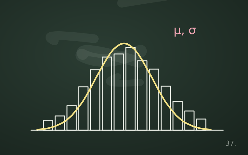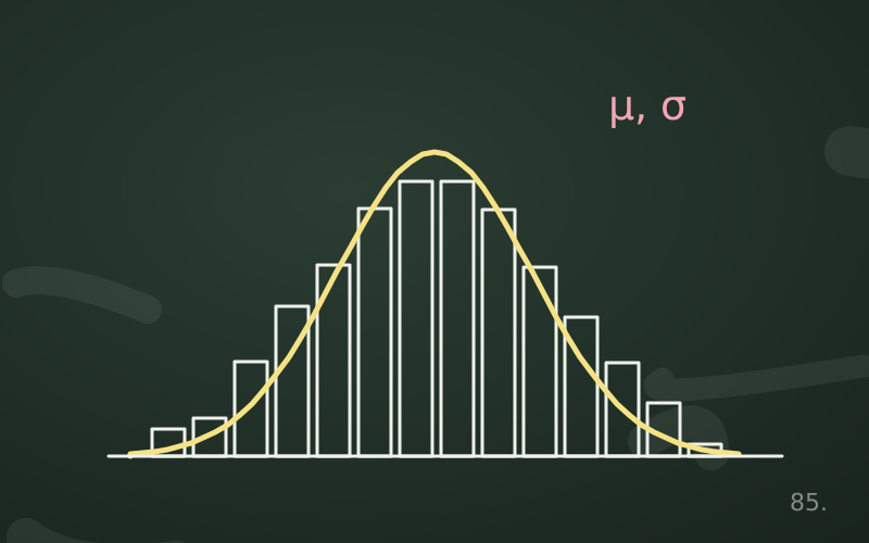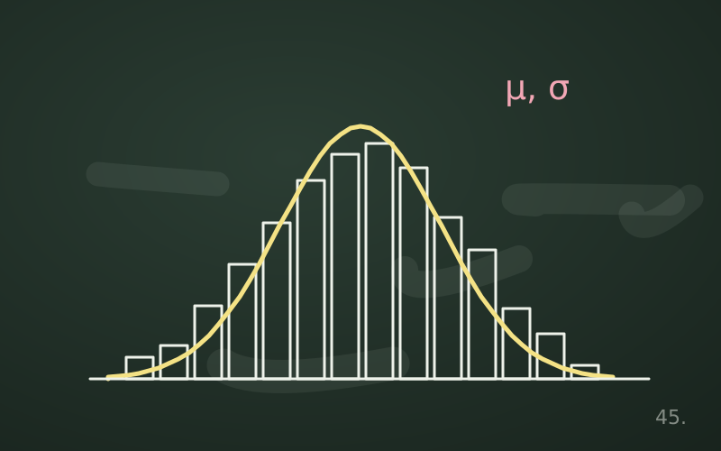
The normal distribution, also called Gaussian, is the famous bell curve. It appears in statistics textbooks, quality control, laboratory measurements and countless models. It really is important, but it is also the most misused distribution. It is worth knowing what it says, how to use it and above all when not to use it.
The main features
A normal distribution is determined by just two parameters:
- the mean μ, which sets the centre of the bell;
- the standard deviation σ, which sets its width.
We write X ~ N(μ, σ²). The curve is symmetric about the mean, so mean, median and mode coincide. The tails fall off very quickly: values far from the mean become extremely rare very fast.
It is a continuous distribution: the probability of a single exact value is zero, and we compute instead probabilities of intervals, which correspond to areas under the curve.
The 68-95-99.7 rule
For any normal distribution these approximate proportions hold:
| Interval | Proportion of values |
|---|---|
| μ ± 1σ | about 68% |
| μ ± 2σ | about 95% |
| μ ± 3σ | about 99.7% |
It follows that a value more than 3 standard deviations from the mean, in either direction, occurs about 3 times in 1,000. To be precise, the interval containing exactly 95% is μ ± 1.96σ; the value 2 is a convenient rounding.
Standardising: z-scores
Every normal can be reduced to the standard normal, with mean 0 and standard deviation 1, by computing:
z = (x − μ) / σ
The z-score tells you how many standard deviations a value lies from the mean. It allows comparison of different quantities: a mark of 27 in an exam with mean 24 and standard deviation 2 has z = 1.5; a score of 80 in a test with mean 70 and standard deviation 10 has z = 1. The first result is relatively more exceptional.
A quality control example
A machine cuts bars with an average length of 50 mm and a standard deviation of 0.2 mm, and the lengths follow a normal distribution well. The specifications accept bars between 49.6 and 50.4 mm. The limits correspond to z = −2 and z = +2, so about 95% of bars conform and about 5% are rejected.
If the tolerance is tightened to ±0.3 mm, that is ±1.5σ, the conforming share drops to about 87%. To get back to 95% the machine's standard deviation would have to be reduced to about 0.15 mm.
Computing with Python
from scipy.stats import norm

mu, sigma = 50, 0.2
inside = norm.cdf(50.4, mu, sigma) - norm.cdf(49.6, mu, sigma)
print(inside)                    # about 0.954
print(norm.ppf(0.99, mu, sigma)) # length exceeded by only 1%
cdf gives the probability of being below a value, ppf does the opposite: given a percentile, it returns the corresponding value.
Why the normal is so widespread
The main reason is the central limit theorem: the sum or average of many small independent influences tends to have an approximately normal distribution, whatever the distribution of the individual influences. Measurement errors, which are often the sum of many small disturbances, behave like this. For the same reason sample means are approximately normal even when the original data are not, and many statistical tests rely on this.
When normality is a mistake
Heavy tails
Many real quantities have much heavier tails than the normal: extreme events happen far more often than the bell predicts. Web service response times are the typical example: most requests are fast, but a minority take much longer. If you estimate the «worst case» as the mean plus three standard deviations, you seriously underestimate real latencies. The same applies to financial price changes and file sizes.
Skewness and natural limits
Times, amounts and counts cannot be negative. If the mean is close to zero and the spread is wide, a normal would assign probability to impossible negative values. In these cases the logarithm of the quantity is often much closer to a normal than the original data.
Mixtures of populations
If two different groups are measured together, for example the performance of two server models, the resulting distribution may have two peaks. Describing it with a single normal hides precisely the most interesting information.
How to check normality
- Look at the data: a histogram immediately shows skewness and multiple peaks.
- Use a quantile-quantile plot: if the points lie on a straight line, normality is plausible; curves at the ends indicate different tails.
- Compare the tails: count how many values exceed 3 standard deviations and compare them with the roughly 0.3% expected.
- Do not rely on formal tests alone: with huge samples they reject normality for irrelevant deviations, with small samples they fail to detect even large ones.
In short
- The normal is defined by mean and standard deviation and is symmetric.
- About 68%, 95% and 99.7% of values fall within 1, 2 and 3 standard deviations.
- Z-scores allow comparison of quantities on different scales.
- The central limit theorem explains why averages tend towards normality.
- Latencies, amounts and heavy-tailed data should not be treated as normal without checking.