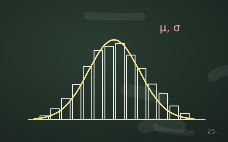
Two servers have the same average response time: 100 milliseconds. The first always responds between 95 and 105, the second swings between 40 and 160. For a user they are very different experiences, but the mean does not say so. Measures of spread complement measures of central tendency: they measure how far the data stray from the centre, and without them any numerical summary is incomplete.
The range
The simplest measure is the range, the difference between the maximum and the minimum value. It is immediate but fragile: it depends on just two values, and a single anomalous data point upends it. It also tends to grow with the number of observations, because the more data you collect, the more likely you are to meet extremes.
Variance and standard deviation
Variance measures the average of the squared deviations from the mean. The standard deviation is its square root and has the advantage of being expressed in the same unit as the data.
Why we divide by n − 1
When computing the variance of a sample to estimate that of the population, the sum of squared deviations is divided by n − 1 instead of n. The reason is that the deviations are computed from the sample mean, which is by construction the point closest to the data themselves: dividing by n would underestimate the variance on average. The correction, known as Bessel's correction, removes this bias. With large samples the difference is negligible, with small samples it is not.
The two-server example
Five measurements for each server, in milliseconds:
- Server A: 95, 98, 100, 102, 105
- Server B: 40, 60, 100, 140, 160
Both have a mean of 100. For A the sum of squared deviations is 25 + 4 + 0 + 4 + 25 = 58; divided by 4 it gives a variance of 14.5 and a standard deviation of about 3.8 ms. For B the sum is 3,600 + 1,600 + 0 + 1,600 + 3,600 = 10,400; divided by 4 it gives 2,600, with a standard deviation of about 51 ms. The number neatly summarises the difference that was evident to the eye.
The limitation
Like the mean, the standard deviation is sensitive to extreme values, even more so, because deviations are squared. A single very distant value can dominate it.
Robust measures
The interquartile range
Quartiles divide the sorted data into four equal parts. The first quartile Q1 has 25% of the data below it, the third quartile Q3 has 75%. The interquartile range is IQR = Q3 − Q1 and measures the width of the middle half of the data, ignoring the tails. It is robust: extreme values do not affect it.
There are slightly different methods for computing quartiles, which give somewhat different results on small samples.
The median absolute deviation
The MAD (median absolute deviation) is computed as follows: find the median of the data, compute the absolute distance of each value from it, and take the median of these distances. It is even more robust than the IQR and is often used to detect anomalies in monitoring data.
Detecting outliers
A very widespread rule, also used in box plots, treats as potentially anomalous the values:
- below Q1 − 1.5 · IQR;
- above Q3 + 1.5 · IQR.
Suppose a service's latencies have Q1 = 40 ms and Q3 = 80 ms. The IQR is 40 ms, so the upper threshold is 80 + 60 = 140 ms. Requests above 140 ms are flagged.
Be careful, though: an outlier is not automatically an error. It may be a measurement error to correct, but also the most important data point in the whole set: the slow request that reveals a problem, the fraudulent transaction, the incipient failure. Removing outliers without understanding them is one of the most common mistakes in data analysis. In forensic analysis work, for example, it is often precisely the out-of-range values that show where to look.
The coefficient of variation
To compare the variability of quantities on different scales, the coefficient of variation is used, the ratio of standard deviation to mean. A standard deviation of 5 ms is huge for a service that responds on average in 10 ms (CV = 50%), negligible for one that responds in 1,000 ms (CV = 0.5%). It only makes sense for positive quantities with a meaningful zero: it should not be used, for example, with temperatures in degrees Celsius.
Summary
| Measure | Robust | Typical use |
|---|---|---|
| Range | No | First look, physical limits |
| Standard deviation | No | Symmetric data, basis of classical methods |
| Interquartile range | Yes | Skewed data, box plots |
| MAD | Yes | Anomaly detection |
| Coefficient of variation | No | Comparisons across different scales |
Good practice
- Always pair a mean with a measure of spread.
- For skewed data use median and IQR instead of mean and standard deviation.
- Before removing an outlier, find out where it comes from.
- State whether the standard deviation is a sample one (n − 1) or a population one (n).
In short
- Spread tells you how far the data stray from the centre and complements the mean.
- Sample variance is divided by n − 1 so as not to underestimate the true one.
- Standard deviation and range are sensitive to extremes; IQR and MAD are not.
- The 1.5 IQR rule flags possible outliers, which must be understood before being discarded.
- The coefficient of variation allows comparisons between quantities on different scales.