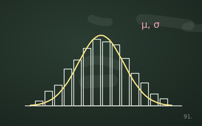
The central limit theorem is the reason much of classical statistics works. It says something surprising: even if individual data points have a strange, skewed or stepped distribution, the mean of a large enough sample has an approximately normal distribution. This is what makes it possible to build confidence intervals and tests without knowing the exact shape of the data.
The statement in plain words
Take n independent observations from the same distribution with mean μ and finite standard deviation σ. Compute their mean. If we repeated the operation a great many times, the means obtained would have a distribution that:
- is centred on μ, the true mean;
- has standard deviation σ / √n, called the standard error;
- becomes more and more like a normal as n grows.
The last point is the heart of the theorem, and it holds whatever the shape of the original distribution, provided the variance is finite.
An example with dice
The result of one die has a flat distribution: each value from 1 to 6 has probability 1/6, no bell at all. But the mean of two dice already has a triangular shape, with 3.5 as the most likely value. The mean of five dice resembles a bell, and the mean of thirty dice is almost indistinguishable from a normal. The mean always stays at 3.5, while the spread narrows: the standard deviation of a single die is about 1.71, that of the mean of 30 dice about 1.71/√30 ≈ 0.31.
A simulation with skewed data
The most instructive example uses highly skewed data, such as a service's response times. Let us simulate them with an exponential distribution with a mean of 200 milliseconds:
import numpy as np

rng = np.random.default_rng(1)
data = rng.exponential(200, size=(10_000, 40))  # 10,000 samples of 40
means = data.mean(axis=1)

print(means.mean())        # about 200
print(means.std())         # about 200 / sqrt(40), i.e. about 31.6
print(np.percentile(means, [2.5, 97.5]))
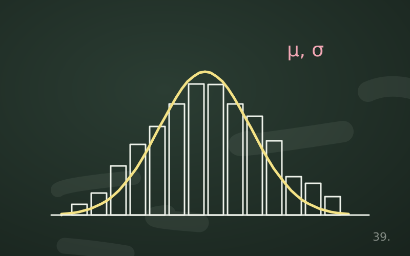
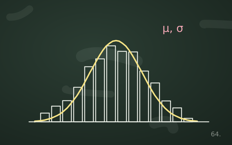
The individual times are strongly skewed: many low values and a long tail to the right. The means of 40 times, by contrast, are distributed almost symmetrically around 200, with a spread of about 31.6. A histogram of the means shows a recognisable bell, with a slight residual skew.
The standard error and the cost of precision
The formula σ / √n has an important practical consequence: the precision of the mean grows with the square root of the number of observations. To halve the standard error it is not enough to double the sample, you have to quadruple it. Going from 100 to 400 measurements halves the uncertainty; halving it again requires 1,600 measurements.
This is why beyond a certain point collecting more data yields less and less, and why it pays to decide in advance what precision is really needed.
Why it matters so much
Thanks to the theorem we can say, to a good approximation, that the sample mean falls within about two standard errors of the true mean in about 95% of samples. From this come:
- confidence intervals for a mean or a proportion;
- tests on means, such as the t-test and the z-test;
- control charts that monitor the mean of a production process;
- the margins of error of opinion polls.
All these tools work even if the original data are not normal, precisely because they operate on means.
When the theorem is not enough
The 30-case rule is not universal
You often read that 30 observations guarantee normality. It is a rule of thumb, not a theorem. With mildly skewed data even fewer cases are enough; with highly skewed or heavy-tailed data many more are needed. Proportions very close to 0 or 1, such as a 0.5% conversion rate, require large samples before the distribution of the proportion becomes symmetric.
Infinite variance
The theorem requires a finite variance. There are distributions, such as the Cauchy distribution, for which the mean of many values does not settle at all: the mean of a thousand observations is as spread out as a single observation. In real data with extremely heavy tails, for example some distributions of amounts or sizes, means converge very slowly and a single value can shift them a great deal.
Non-independent data
If observations are correlated with each other, such as consecutive measurements over time or users in the same group, the real standard error is larger than σ / √n. Using the classical formula leads to intervals that are too narrow and to false confidence.
It concerns means, not individual data
The theorem does not say that data become normal with a large sample. Response times remain skewed even with a million measurements; it is their mean that behaves well. For estimating the 99th percentile of latency the central limit theorem does not help.
In short
- The mean of many independent observations tends towards a normal distribution.
- The standard error of the mean is σ / √n: halving it requires a sample four times larger.
- Confidence intervals, tests and margins of error rest on this result.
- Highly skewed data, infinite variance or dependent observations limit its use.
- The theorem concerns means, not the distribution of individual data points.