Much data consists not of measurements but of counts in categories: how many times each face of a die comes up, how many errors per browser type, how many customers per satisfaction band. To ask whether these counts are compatible with a hypothesis, the classic tool is the chi-square test. It is easy to compute even by hand and teaches the logic of tests well: compare what you observe with what you would expect.
The basic idea
For each category you compare the observed frequency O with the expected frequency E under the null hypothesis, and add up the deviations like this:
χ² = Σ (O − E)² / E
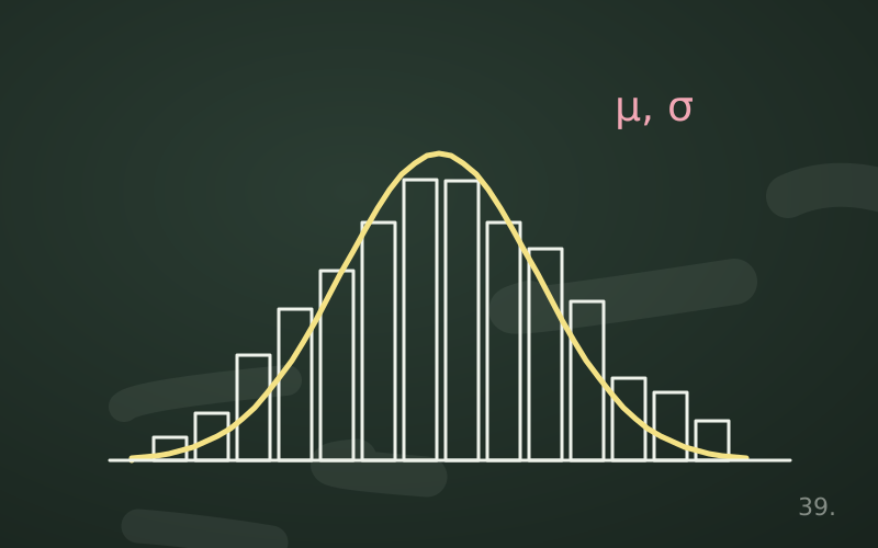
The deviations are squared, so positive and negative ones do not cancel out, and divided by the expected value, so a deviation of 10 weighs more in a category that expected 20 than in one that expected 1,000. If the null hypothesis is true, the statistic approximately follows a chi-square distribution with a certain number of degrees of freedom. Large values indicate deviations that are hard to attribute to chance.
First use: goodness-of-fit test
The goodness-of-fit test checks whether an observed distribution is compatible with a theoretical one.
Is the die fair?
We roll a die 120 times. If it is fair, we expect 20 occurrences per face.
| Face | 1 | 2 | 3 | 4 | 5 | 6 |
|---|---|---|---|---|---|---|
| Observed | 15 | 22 | 18 | 25 | 17 | 23 |
| Expected | 20 | 20 | 20 | 20 | 20 | 20 |
| (O − E)² / E | 1.25 | 0.20 | 0.20 | 1.25 | 0.45 | 0.45 |
The sum is χ² = 3.8. The degrees of freedom are the number of categories minus one, that is 5: once five counts and the total are fixed, the sixth is determined. With 5 degrees of freedom, a value of 3.8 corresponds to a p-value of about 0.58. The observed fluctuations are entirely normal for a fair die.
This example also shows how easy it is to see patterns in noise: the 4 came up 25 times and the 1 only 15, a difference that looks remarkable to the eye but that chance produces frequently.
Second use: test of independence
The test of independence checks whether two categorical variables are associated. The data are organised in a contingency table.
Do errors depend on the browser?
We analyse 3,000 sessions of a web application, a thousand for each of three browsers:
| With error | Without error | Total | |
|---|---|---|---|
| Browser A | 30 | 970 | 1,000 |
| Browser B | 50 | 950 | 1,000 |
| Browser C | 40 | 960 | 1,000 |
| Total | 120 | 2,880 | 3,000 |
If error and browser were independent, every browser would have the same overall error rate, 120/3,000 = 4%. Expected frequencies are computed as row total × column total / grand total: 40 errors and 960 error-free sessions for each browser.
- Contributions from errors: 10²/40 + 10²/40 + 0 = 5.0.
- Contributions from error-free sessions: 10²/960 + 10²/960 + 0 ≈ 0.21.
- χ² ≈ 5.21.
The degrees of freedom are (rows − 1) × (columns − 1) = 2 × 1 = 2. The p-value is about 0.074. With α = 0.05 independence is not rejected: the difference between browser A's 3% and browser B's 5% could be due to chance. With ten times as many sessions and the same rates, however, the difference would be clearly significant.
With Python
from scipy.stats import chi2_contingency

table = [[30, 970], [50, 950], [40, 960]]
chi2, p, dof, expected = chi2_contingency(table)
print(chi2, p, dof)
For 2 × 2 tables the function applies Yates' correction by default, which makes the test somewhat more conservative; it can be turned off with correction=False.
Conditions of use
The test relies on an approximation that works only if:
- the observations are independent: each unit appears only once in the table;
- the data are counts, not percentages or means: applying the test to percentages gives meaningless results;
- the expected frequencies are not too small: a common rule of thumb asks for them to be at least 5 in the great majority of cells.
When expected frequencies are small, for example in 2 × 2 tables with few cases, Fisher's exact test is used, which does not rely on the approximation.
What the test does not tell you
- It does not measure the strength of the association. With huge samples even weak associations come out significant. For strength, indices such as Cramér's V are used or, more simply, a direct comparison of percentages.
- It does not say where the difference lies. A significant χ² in a large table indicates that some cell departs from expectation; to understand which, you must look at the contributions of individual cells or at standardised residuals.
- It does not establish a causal link. If errors are more frequent with one browser, the cause may be the browser itself, but also the type of users or devices that use it.
In short
- Chi-square compares observed and expected frequencies in categories.
- The goodness-of-fit test checks a theoretical distribution, the independence test an association.
- Degrees of freedom are k − 1 for goodness of fit and (r − 1)(c − 1) for independence.
- It should be applied to independent counts with expected frequencies that are not too small.
- A significant result indicates neither the strength nor the cause of the association.