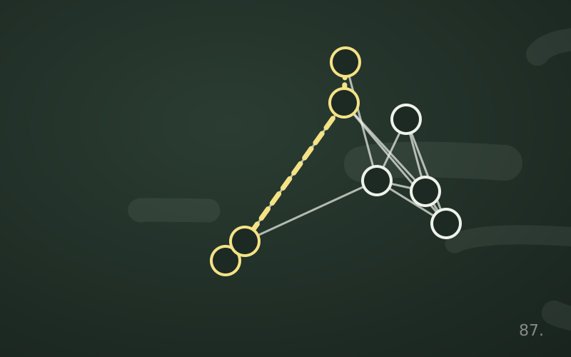
Anyone exploring a cave with a ball of string follows a precise method: take a tunnel and keep going as far as possible; on reaching a dead end, go back along the string to the last fork with an unexplored passage, and set off again from there. This is exactly the strategy of depth-first search, or DFS.
While breadth-first search proceeds in concentric rings, DFS goes «deep» along one branch before considering the alternatives. It does not find shortest paths, but it reveals the structure of the graph: components, cycles, critical points, dependency orders.
Recursion or stack
The most natural form of DFS is recursive:
def dfs(adj, u, visited):
    visited.add(u)
    for v in adj[u]:
        if v not in visited:
            dfs(adj, v, visited)
Recursion implicitly uses the call stack: each pending call is a fork to come back to. On large graphs, however, the recursion depth can exceed the language's limit (in Python the default limit is around a thousand calls). In those cases an explicit stack is used:
def dfs_iterative(adj, s):
    visited = set()
    stack = [s]
    while stack:
        u = stack.pop()
        if u in visited:
            continue
        visited.add(u)
        for v in adj[u]:
            if v not in visited:
                stack.append(v)
    return visited
Notice the difference from BFS: simply replacing the queue with a stack (last in, first out) completely changes the character of the exploration. Here the check happens when a vertex is popped, because it may be pushed several times before being visited.
The cost remains proportional to n + m with adjacency lists.
Discovery and finish times
DFS becomes truly powerful when two moments are recorded for each vertex: when it is discovered (the call is entered) and when it is finished (all its neighbours have been explored and the call returns). With a global counter you get two numbers, d[u] and f[u].
These intervals nest like parentheses: for any two vertices, either one interval entirely contains the other (one is a descendant of the other in the DFS tree), or the two intervals are disjoint. This property underpins topological sorting and the algorithms for strongly connected components.
Classifying edges
While traversing a directed graph, every edge (u, v) falls into one of four categories:
- tree edge: v is discovered precisely through this edge;
- back edge: v is an ancestor of u still being visited;
- forward edge: v is an already finished descendant of u;
- cross edge: v is in another, already finished branch.
The category that matters most is the second: a directed graph contains a cycle if and only if DFS finds at least one back edge.
Detecting cycles in practice
For a directed graph three colours are used: white (never seen), grey (being visited, that is, on the current stack), black (finished). If, while visiting u, you meet a grey neighbour, you have found a cycle.
This is the same check that build systems and package managers perform when they report a «circular dependency»: package A requires B, B requires C, C requires A. By rebuilding the chain of grey vertices you can also show the user the exact cycle, which is far more useful than a generic error message.
In undirected graphs it is enough to remember the vertex you came from: an already visited neighbour that is not the parent indicates a cycle.
Connected components
In an undirected graph, a DFS launched from a vertex visits exactly its connected component. To find them all, walk through the list of vertices and start a new traversal from every vertex not yet reached, assigning a different component number at each start.
Concrete examples:
- in a binary image, blobs of adjacent pixels of the same colour are connected components (this is the principle behind the «bucket fill» tool in graphics programs);
- in a set of accounts linked by shared email addresses or devices, each component groups the accounts that probably belong to the same person or organisation;
- in an electrical or water network, the components show which areas are left isolated after a failure.
Bridges and articulation points
Using discovery times you can also compute, for each vertex, the lowest discovery time reachable from its subtree using at most one back edge. From this value you derive bridges (edges whose removal disconnects the graph) and articulation points (vertices with the same property). In a company network these are the links and devices that represent a single point of failure: knowing where they are is the first step towards adding redundancy.
In short
- DFS explores one branch to the end before backtracking, using recursion or an explicit stack.
- The cost is proportional to n + m; on deep graphs the iterative version is safer.
- Discovery and finish times form nested intervals, the basis of many other algorithms.
- A back edge signals a cycle: this is the circular-dependency check.
- Connected components, bridges and articulation points can all be found with a DFS.