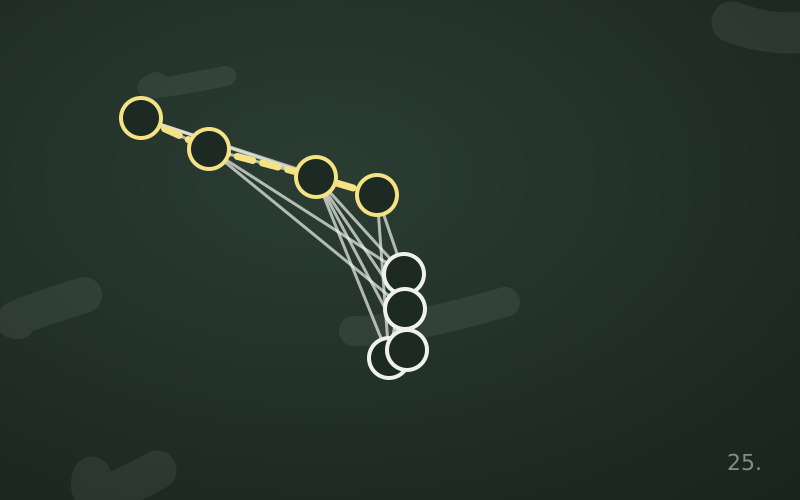
Imagine throwing a stone into a pond: the waves spread out in concentric circles, reaching nearby points first and distant ones later. Breadth-first search, known by its acronym BFS, explores a graph in exactly this way. It starts from a vertex, visits all its neighbours, then the neighbours of the neighbours, and so on, one «ring» at a time.
It is one of the simplest graph algorithms and, at the same time, one of the most widely used. It has a valuable property: in a graph without weights it finds the paths with the fewest edges.
The idea: a queue
The heart of BFS is a queue (FIFO, first in, first out). The scheme is:
- put the starting vertex in the queue and mark it as visited;
- while the queue is not empty, take out the first vertex u;
- for each neighbour v of u not yet visited, mark it as visited, remember that you reached it from u and add it to the back of the queue.
Because the queue serves vertices in order of arrival, all vertices at distance 1 are taken out before those at distance 2, which in turn come before those at distance 3.
from collections import deque

def bfs(adj, s):
    dist = {s: 0}
    parent = {s: None}
    queue = deque([s])
    while queue:
        u = queue.popleft()
        for v in adj[u]:
            if v not in dist:
                dist[v] = dist[u] + 1
                parent[v] = u
                queue.append(v)
    return dist, parent
A detail that often makes the difference: a vertex should be marked as visited when it enters the queue, not when it leaves. Otherwise the same vertex can be added several times, wasting time and memory.
Rebuilding the path
The parent dictionary records, for each vertex reached, which vertex it was reached from. To rebuild the shortest path from s to a target t, start from t and walk back from parent to parent until s, then reverse the sequence. The set of edges (parent[v], v) forms a tree, called the BFS tree, which contains a shortest path from s to every reachable vertex.
How much it costs
Each vertex enters the queue at most once and, when it leaves, its neighbours are scanned. With adjacency lists the total cost is proportional to n + m: linear in the size of the graph. With an adjacency matrix it becomes n², because finding the neighbours requires scanning a whole row.
The extra memory is dominated by the queue and the dictionaries, so it is proportional to n. On very «wide» graphs, where one level contains a great many vertices, the queue can grow large: this is the main drawback of BFS compared with depth-first search.
Why it finds shortest paths
This can be proved by induction on the levels: when a vertex v is discovered for the first time from u, dist[u] is already the minimum distance of u, and no vertex at a smaller distance is left to explore. Therefore dist[u] + 1 is the minimum distance of v.
Be careful, though: the guarantee holds only if all edges «cost» the same. If edges have different weights, the path with fewer edges may be longer in kilometres or time. In that case you need Dijkstra's algorithm, which can be seen as a BFS where the plain queue is replaced by a priority queue.
Concrete uses
- Mazes and grids: each cell is a vertex and the neighbours are the adjacent free cells. BFS finds the route to the exit with the fewest steps.
- Degrees of separation: in a social network, the BFS distance between two people is the minimum number of intermediaries.
- Network reachability: starting from a compromised host, a BFS over the graph of possible connections shows which systems can be reached in one, two or three hops. During incident analysis it is an orderly way to establish the scope.
- Web crawlers: exploring a site level by level from the home page makes it possible to limit depth and prioritise the pages closest to the start.
- Bipartite graphs: by colouring the BFS levels alternately with two colours, you find out whether the graph is bipartite. If an edge joins two vertices of the same colour, it is not.
Useful variants
Multi-source BFS
Several starting vertices are put in the queue at the beginning, all at distance 0. The result is, for each vertex, the distance from the nearest source: for example the distance of each house from the nearest pharmacy.
0-1 BFS
If edges weigh only 0 or 1, a double-ended queue is used: weight-0 edges push to the front, weight-1 edges to the back. You get shortest paths in linear time, without Dijkstra's priority queue.
Bidirectional BFS
The search starts simultaneously from the source and the destination and stops when the two explorations meet. In graphs with many neighbours per node it drastically reduces the number of vertices visited.
In short
- BFS explores the graph level by level using a FIFO queue.
- In unweighted graphs it finds the paths with the fewest edges.
- The cost is proportional to n + m with adjacency lists.
- Each vertex should be marked as visited when it enters the queue, not when it leaves.
- Variants such as multi-source, 0-1 and bidirectional BFS cover many practical cases.