How many defective parts will I find in a batch of 20? How many users out of 50 will click a button? How many correct answers will someone give by guessing on a multiple-choice test? They are all questions of the same type: counting how many times an event occurs in a fixed number of attempts. The answer is the binomial distribution, one of the most widely used in statistics.
Conditions of applicability
The binomial describes the number of successes X in n trials when four conditions hold:
- the number of trials n is fixed in advance;
- each trial has only two outcomes, conventionally «success» and «failure»;
- the probability of success p is the same in every trial;
- the trials are independent of each other.
Each individual trial is called a Bernoulli trial. We write X ~ Bin(n, p).
The conditions must really be checked. If we draw without replacement from a small batch, the probability changes with every draw and independence breaks down; in that case the correct model is the hypergeometric. If the batch is very large compared with the sample, however, the binomial remains an excellent approximation.
The formula
The probability of getting exactly k successes is:
P(X = k) = C(n, k) · pᵏ · (1 − p)ⁿ⁻ᵏ
where C(n, k) = n! / (k! (n − k)!) is the binomial coefficient. The logic is clear if you read it piece by piece:
- pᵏ · (1 − p)ⁿ⁻ᵏ is the probability of one particular sequence with k successes and n − k failures;
- C(n, k) counts how many different sequences have exactly k successes.
A small example
We toss a fair coin 4 times. What is the probability of getting exactly 2 heads? The sequences with two heads number C(4, 2) = 6 (HHTT, HTHT, HTTH, THHT, THTH, TTHH), each with probability (1/2)⁴ = 1/16. So P(X = 2) = 6/16 = 0.375.
Mean and variance
For the binomial there is no need to add up all the cases: thanks to linearity of expectation we get straight away
- mean: E[X] = n · p
- variance: Var(X) = n · p · (1 − p)
The reason is that X is the sum of n independent variables that equal 1 with probability p and 0 otherwise; each has mean p and variance p(1 − p).
The variance is largest when p = 0.5 and shrinks as p approaches 0 or 1: if an event is almost certain or almost impossible, there is little uncertainty about the number of successes.
A full example: quality control
A process produces parts with a 5% probability of defect. A sample of 20 parts is drawn from a large production run. Let us compute some probabilities.
- No defects: P(X = 0) = 0.95²⁰ ≈ 0.358.
- Exactly one defect: P(X = 1) = 20 · 0.05 · 0.95¹⁹ ≈ 0.377.
- Exactly two defects: P(X = 2) = 190 · 0.05² · 0.95¹⁸ ≈ 0.189.
- Three or more defects: 1 − (0.358 + 0.377 + 0.189) ≈ 0.075.
The expected mean is 20 · 0.05 = 1 defect, with a standard deviation of √(20 · 0.05 · 0.95) ≈ 0.97.
These numbers are the basis of a sampling plan. If the rule is «reject the batch when I find three or more defects», a process running normally at 5% is still rejected about 7.5 times out of 100. It is a type I error, and knowing its frequency lets you choose the threshold deliberately.
Computing with Python
With the SciPy library the calculations become immediate:
from scipy.stats import binom

n, p = 20, 0.05
print(binom.pmf(0, n, p))      # P(X = 0)
print(binom.cdf(2, n, p))      # P(X <= 2)
print(binom.sf(2, n, p))       # P(X > 2), i.e. P(X >= 3)
print(binom.mean(n, p), binom.std(n, p))
The sf function (survival function) computes the right tail directly and is more accurate than 1 - cdf when probabilities are extremely small.
Common mistakes
- Forgetting the binomial coefficient: the probability of 2 heads in 4 tosses is not (1/2)⁴, because there are six favourable sequences.
- Confusing «exactly» with «at least»: «at least 3» requires adding P(3), P(4) and so on, or using the complement.
- Applying it to dependent trials: users in the same office, failures from the same batch or answers that influence each other violate independence and make the real variance larger than n · p · (1 − p).
- Using a non-constant p: if the click probability varies a lot between groups of users, lumping them all into a single binomial hides the heterogeneity.
Links with other distributions
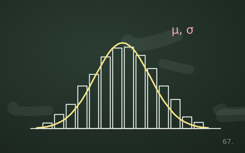
When n is large and p is small, the binomial is well approximated by the Poisson distribution with parameter λ = n · p. When instead n is large and p is not too close to 0 or 1, the shape of the binomial approaches that of the normal, with the same mean and variance. These approximations were essential when calculations were done by hand and remain useful for quick reasoning.
In short
- The binomial counts successes in n independent trials with the same probability p.
- P(X = k) combines the number of favourable sequences and the probability of each.
- Mean n · p and variance n · p · (1 − p) are obtained without long calculations.
- In a sampling plan the binomial tells you how often a good batch is rejected.
- Dependent trials or a varying p make the model inadequate.