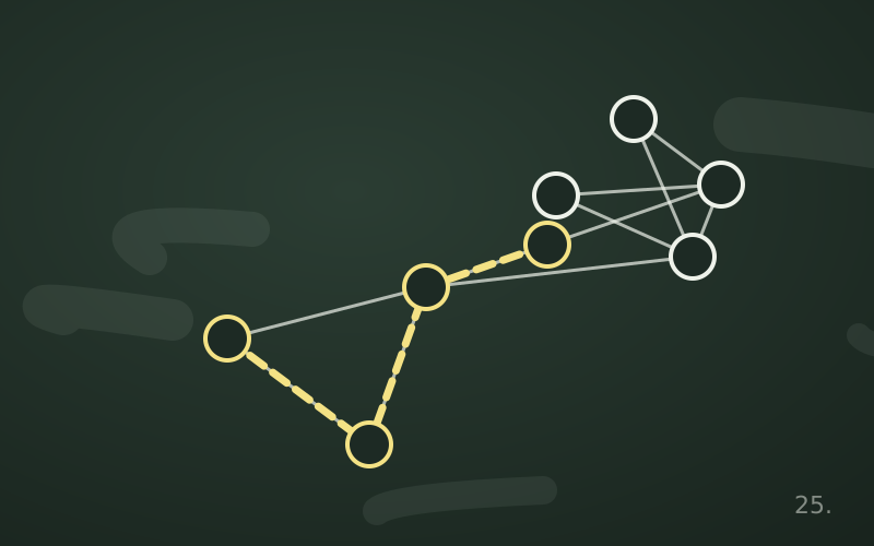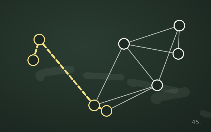
In an undirected graph, connectivity is simple: two vertices are in the same component if there is a path between them. In directed graphs things get more complicated, because being able to go from A to B does not mean being able to come back from B to A. A web page can link to another without being cited in return; a software module can import another without being imported by it.
Strongly connected components (SCCs) answer the right question for directed graphs: which groups of vertices are all mutually reachable?
Definition
Two vertices u and v are strongly connected if there is a directed path from u to v and also one from v to u. This relation is reflexive, symmetric and transitive, so it divides the vertices into classes: the strongly connected components.
Examples:
- in a dependency graph between modules, an SCC with more than one element is a group of modules that import one another circularly;
- in a network of accounts transferring money, an SCC is a group in which money can circulate and return to its starting point;
- in an automaton, an SCC is a set of states that can be left but in which, once you return, you can loop indefinitely.
The condensed graph
If each SCC is contracted into a single «supervertex», keeping the edges between different components, you obtain the condensed graph (or condensation). This graph is always a DAG: if there were a cycle between two components, their vertices would be mutually reachable and would therefore belong to the same component.
This is a very practical result. Many hard problems on graphs with cycles become simple on DAGs, thanks to topological sorting. The standard strategy is therefore: find the SCCs, solve the problem inside each component (where everything is reachable from everything), then propagate the results across the condensed DAG in topological order.
Kosaraju's algorithm
It is the easiest to understand and requires two depth-first searches.
- Run a complete DFS on the graph and record the order in which vertices finish.
- Build the transposed graph, reversing the direction of every edge.
- Run DFS on the transposed graph, taking starting vertices in decreasing finish order. Each traversal launched in this phase reaches exactly one strongly connected component.
Why does it work? The vertex that finishes last in the first DFS belongs to a «source» component of the condensed DAG, from which there is no way back. In the transposed graph this component becomes a «sink»: starting there, the traversal cannot get out and collects only its own component. Then you move on to the next component in the order, and so on.
The cost is proportional to n + m, at the price of also building and storing the transposed graph.
Tarjan's algorithm
Tarjan finds the same components with a single DFS and no transposed graph. For each vertex it keeps two values:
- index: the discovery order;
- lowlink: the smallest index reachable from the vertex's subtree, using tree edges and at most one edge to a vertex still on the stack.
Vertices are pushed onto a stack as they are discovered. When, at the end of the visit of a vertex v, lowlink[v] = index[v], v is the «root» of a component: all vertices are popped from the stack down to and including v, and they form the component.
def tarjan(adj, n):
    index, low = [None] * n, [0] * n
    on_stack, stack, components = [False] * n, [], []
    counter = [0]
    def visit(v):
        index[v] = low[v] = counter[0]; counter[0] += 1
        stack.append(v); on_stack[v] = True
        for w in adj[v]:
            if index[w] is None:
                visit(w)
                low[v] = min(low[v], low[w])
            elif on_stack[w]:
                low[v] = min(low[v], index[w])
        if low[v] == index[v]:
            comp = []
            while True:
                w = stack.pop(); on_stack[w] = False
                comp.append(w)
                if w == v: break
            components.append(comp)
    for v in range(n):
        if index[v] is None:
            visit(v)
    return components
Tarjan also costs n + m. A useful detail: components are produced in reverse topological order of the condensed graph, so an extra sort is often unnecessary. On large graphs it should be rewritten iteratively to avoid exceeding the recursion limit.
Comparison
| Aspect | Kosaraju | Tarjan |
|---|---|---|
| DFS passes | two | one |
| Transposed graph | required | not required |
| Ease of understanding | high | medium |
| Order of components | topological | reverse topological |
An elegant application: 2-SAT
A 2-SAT problem asks you to assign true or false to variables while respecting clauses such as «x or not y». Each clause becomes two implications, and therefore two edges in an implication graph. The formula is satisfiable if and only if no variable lies in the same SCC as its own negation. The components also yield a valid assignment. A logic problem is thus solved in linear time with a graph traversal.
In short
- In directed graphs, an SCC gathers vertices that are mutually reachable.
- Contracting the SCCs always yields a DAG, on which many problems become simple.
- Kosaraju uses two DFS passes and the transposed graph; it is the most intuitive.
- Tarjan uses a single DFS with indices and lowlinks; it outputs components in reverse topological order.
- Both cost n + m and solve, among other things, the 2-SAT problem.