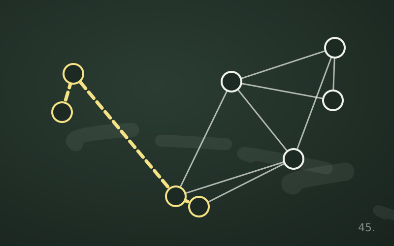
Dijkstra's algorithm is fast and elegant, but it has a clear limit: all edges must have non-negative weight. When this condition does not hold, a more patient approach is needed. The Bellman-Ford algorithm is slower, but it accepts negative weights and, above all, it can recognise the situation in which the problem itself makes no sense: the presence of a negative cycle.
When negative weights appear
A road length is never negative, but many problems modelled as shortest paths are:
- gains and costs: in a sequence of operations some cost money and others earn it; a gain is represented as a negative weight;
- difference constraints: systems of constraints such as «event B must happen at most 3 hours after A» translate into a graph where some edges have negative weight, and the solutions are given precisely by shortest distances;
- exchange rates: by using logarithms, as we shall see, the search for arbitrage opportunities becomes a search for negative cycles.
The idea: relax everything, several times
Bellman-Ford does not choose a clever order in which to process vertices. It relaxes all edges, then does it again, and again, n − 1 times in total.
def bellman_ford(n, edges, s):
    INF = float("inf")
    dist = [INF] * n
    dist[s] = 0
    for _ in range(n - 1):
        changed = False
        for u, v, w in edges:
            if dist[u] != INF and dist[u] + w < dist[v]:
                dist[v] = dist[u] + w
                changed = True
        if not changed:
            break
    for u, v, w in edges:
        if dist[u] != INF and dist[u] + w < dist[v]:
            raise ValueError("negative cycle reachable from the source")
    return dist
Why exactly n − 1 passes? If there are no negative cycles, a shortest path does not repeat vertices, so it uses at most n − 1 edges. After the first pass, the distances of all vertices reachable with one edge along a shortest path are correct; after the second, those with two edges; after the k-th, those with k edges. After n − 1 passes, all of them.
The changed variable is an important practical optimisation: if no estimate improves during a pass, subsequent passes would change nothing and we can exit immediately. On many real graphs the algorithm finishes after just a few passes.
The final check: negative cycles
A negative cycle is a cycle whose total weight is less than zero. If it is reachable from the source, going round it once more always lowers the cost, so the «shortest distance» does not exist: you can keep descending forever.
Bellman-Ford detects it with one extra pass. If after n − 1 passes some edge can still be relaxed, there must be a negative cycle. By following the predecessor pointers backwards from the improved vertex for n steps, you are guaranteed to end up inside the cycle, and from there you can rebuild it to show it.
An example: currency arbitrage
Suppose we know the exchange rates between some currencies. An arbitrage is a sequence of conversions that, starting from one currency, returns to the same one with more money than before: the product of the rates along the cycle is greater than 1.
The trick is to turn products into sums with logarithms. Give each edge from X to Y the weight −log(rate X→Y). The product of rates around a cycle is greater than 1 exactly when the sum of the logarithms is positive, that is, when the sum of the weights is negative. Looking for an arbitrage therefore means looking for a negative cycle, a task tailor-made for Bellman-Ford.
In reality, fees, spreads and latency shrink these opportunities, but the model remains a clear example of how transforming the weights reduces a new problem to a known algorithm.
Cost and comparison with Dijkstra
Each pass examines all m edges and there are at most n − 1 passes, so the worst-case cost is proportional to n · m. That is much more than Dijkstra, which costs roughly (n + m) log n.
| Aspect | Dijkstra | Bellman-Ford |
|---|---|---|
| Negative weights | no | yes |
| Detects negative cycles | no | yes |
| Typical cost | (n + m) log n | n · m |
| Data structure | priority queue | edge list |
The practical rule is simple: if all weights are non-negative, use Dijkstra; otherwise Bellman-Ford, or one of its variants.
Variants and uses
- Queue of modified vertices: instead of relaxing every edge on each pass, only the vertices whose estimate has changed are reprocessed. In average cases it speeds things up considerably, although the worst case remains the same.
- Johnson's algorithm: to compute all-pairs shortest paths in sparse graphs with negative weights, Bellman-Ford is used once to «reweight» the edges so they become non-negative, then Dijkstra is run from every vertex.
- Distance-vector routing: some historical network protocols, such as RIP, are based on a distributed version of the same idea: each router tells its neighbours its own estimates and updates them based on those it receives.
In short
- Bellman-Ford computes single-source shortest paths even with negative weights.
- It relaxes all edges for n − 1 passes, stopping early if nothing changes.
- One extra pass reveals negative cycles, where no shortest distance exists.
- With weights −log(rate), searching for arbitrage becomes searching for negative cycles.
- It costs n · m: use it when negative weights are really present.