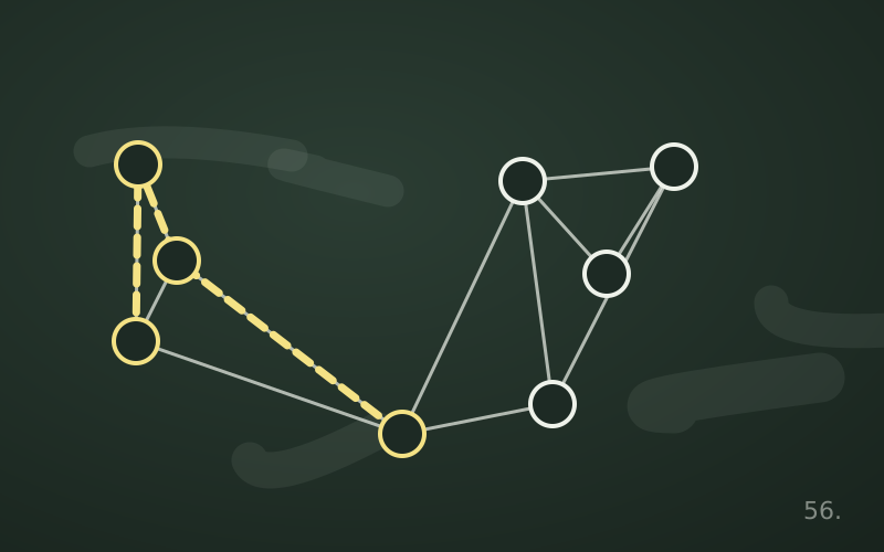
On paper a graph is a drawing of dots and lines. In a program, however, it has to become a data structure, and the choice is not neutral: the same algorithm can take seconds or hours depending on how the graph is stored. There are three classic representations, and each one answers different questions well.
Below, n is the number of vertices and m the number of edges. Assume vertices are numbered from 0 to n − 1: if the data gives them names (cities, IP addresses, usernames), the first step is to build a dictionary that maps each name to an integer.
The adjacency matrix
It is an n × n table in which cell (i, j) is 1 if there is an edge from i to j and 0 otherwise. In weighted graphs the cell holds the weight, and a special value (for example infinity) marks a missing edge. In undirected graphs the matrix is symmetric.
Advantages:
- checking whether two vertices are connected costs a single access, that is, constant time;
- adding or removing an edge is immediate;
- it lends itself to algebraic operations: multiplying the matrix by itself counts the paths of length 2.
The drawback is memory: it needs n² cells regardless of the number of edges. With 100,000 vertices that is 10 billion cells, even if each vertex has barely a dozen neighbours. Moreover, listing the neighbours of a vertex requires scanning a whole row, that is, n operations.
The matrix is therefore worth it for small or dense graphs, and for algorithms that use it directly, such as Floyd-Warshall for all-pairs shortest paths.
Adjacency lists
For each vertex we keep the list of its neighbours. In Python the simplest form is a list of lists:
n = 5
adj = [[] for _ in range(n)]
edges = [(0, 1), (0, 2), (1, 3), (3, 4)]
for u, v in edges:
    adj[u].append(v)
    adj[v].append(u)   # omit this line if the graph is directed
In weighted graphs each element becomes a (neighbour, weight) pair.
Advantages:
- memory is proportional to n + m, which makes it ideal for sparse graphs, that is, almost all real ones;
- iterating over the neighbours of a vertex costs as much as its degree, and that is exactly the operation used by breadth-first and depth-first search, Dijkstra and Prim.
The price is that checking whether a specific edge exists requires scanning the list. If this question is frequent, sets can be used instead of lists, giving an average constant-time check in exchange for a little more memory.
The edge list
It is the most spartan representation: a plain list of (u, v) pairs, or (u, v, weight) triples. It is exactly the format of a CSV file exported from a database or a network analysis tool.
It does not let you find the neighbours of a vertex quickly, but it is perfect when the algorithm has to examine all edges in bulk. Kruskal's algorithm sorts the edges by weight and walks through them; Bellman-Ford repeats a pass over all edges several times. In both cases the edge list is the natural choice.
Quick comparison
| Operation | Matrix | Adjacency lists | Edge list |
|---|---|---|---|
| Memory | n² | n + m | m |
| Does edge (u, v) exist? | constant | degree of u | m |
| List neighbours of u | n | degree of u | m |
| Add an edge | constant | constant | constant |
A compact variant for large graphs
When the graph is static and very large, lists of lists waste memory on pointers and scatter the data. The CSR format (Compressed Sparse Row) is used instead: a single array with all neighbours concatenated, vertex after vertex, and a second array of n + 1 indices saying where each vertex's section starts. The neighbours of u lie between positions index[u] and index[u + 1]. It is the same scheme used for sparse matrices in scientific computing, and it is much faster to scan because the data is contiguous in memory.
How to choose in practice
A few rules that work almost every time:
- Start with adjacency lists: they are the right default for most problems.
- Use the matrix if n is small (a few thousand at most) or if the graph is nearly complete.
- Keep the edge list as the input and output format, and for algorithms that work «edge by edge».
- Move to CSR or specialised libraries when the graph exceeds millions of edges and does not change over time.
Many real programs keep several representations at once: for example adjacency lists for traversals and a set of pairs to quickly answer the question «are these two nodes connected?».
In short
- The adjacency matrix answers in constant time whether an edge exists, but takes n² cells.
- Adjacency lists use space proportional to n + m and are the default choice for sparse graphs.
- The edge list is ideal for raw data and for algorithms such as Kruskal and Bellman-Ford.
- For large, static graphs the CSR format reduces memory and access times.
- The right representation depends on the questions the algorithm will ask most often.