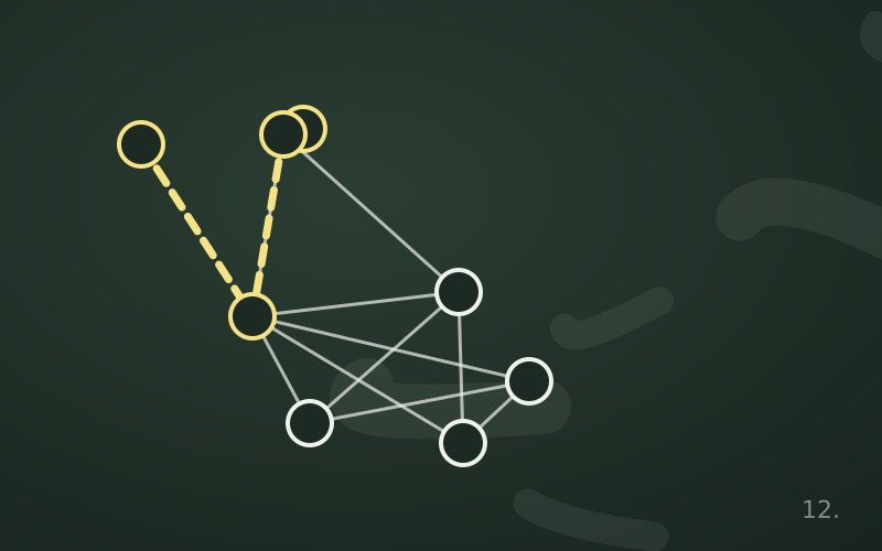
A company has to connect eight buildings on a campus with fibre. Each possible route has a different digging cost. A direct link between every pair of buildings is not needed: it is enough for each one to be reachable from all the others, possibly through intermediate buildings. Which routes should be built to spend as little as possible?
The answer is a minimum spanning tree (MST). It is one of the rare optimisation problems in which a greedy approach, that is, choosing at each step the option that looks best, is guaranteed to reach the optimal solution.
Definitions
Given an undirected, connected, weighted graph:
- a spanning tree is a subset of edges that connects all vertices without forming cycles; with n vertices it contains exactly n − 1 edges;
- a minimum spanning tree is the one with the lowest total weight.
If the graph is not connected we speak of a minimum spanning forest, one tree per component.
The cut property
All MST algorithms rest on a single idea. Split the set of vertices into any two parts; among the edges that cross the split, the one with minimum weight belongs to some minimum spanning tree.
The reason: if a tree did not contain that edge, adding it would create a cycle that crosses the split at least once more, through a heavier edge. Removing the latter would give a tree whose cost is no higher. Kruskal's and Prim's algorithms are two different ways of applying this property repeatedly.
Kruskal's algorithm
- Sort all edges by increasing weight.
- Go through them one at a time: add the edge to the tree if it connects two vertices that are not yet connected; otherwise discard it, because it would create a cycle.
- Stop when you have n − 1 edges.
The delicate point is step 2: how can you quickly tell whether two vertices are already connected? The answer is the union-find structure (or disjoint sets), which maintains a partition of the vertices and offers two operations: finding the representative of a vertex's set and merging two sets.
def kruskal(n, edges):
    parent = list(range(n))
    def find(x):
        while parent[x] != x:
            parent[x] = parent[parent[x]]   # path compression
            x = parent[x]
        return x
    tree, total = [], 0
    for w, u, v in sorted(edges):
        ru, rv = find(u), find(v)
        if ru != rv:
            parent[ru] = rv
            tree.append((u, v, w))
            total += w
    return tree, total
With path compression and union by size or rank, the operations cost almost constant time in practice. The dominant cost becomes the sort: roughly m log m.
Prim's algorithm
Prim grows a single tree starting from any vertex. At each step it adds the lightest edge connecting a vertex already in the tree to one still outside. The cut property applies to the split between «inside» and «outside».
The implementation looks very much like Dijkstra: a priority queue holds the outside vertices, with priority equal to the weight of the best edge linking them to the tree, not the distance from the source. With a binary heap the cost is roughly (n + m) log n.
Which one to choose
| Situation | Recommended choice |
|---|---|
| Edges already in a list, sparse graph | Kruskal |
| Dense graph or matrix representation | Prim with an array, cost n² |
| You also want to know which groups form along the way | Kruskal |
| Edges generated on the fly from neighbours | Prim |
In many practical cases the differences are small; Kruskal is easier to write without bugs.
An example
Four buildings A, B, C, D. Costs: A–B 3, A–C 1, B–C 7, B–D 5, C–D 4. Kruskal sorts: A–C (1), A–B (3), C–D (4), B–D (5), B–C (7). It takes A–C, then A–B, then C–D; at that point it has 3 edges and stops. Total cost 8. B–D and B–C are discarded because they would close cycles.
Concrete applications
- Network design: cables, pipes, power lines, where what matters is the overall connection cost and not the distance between two specific points.
- Clustering: once the MST is built on points with weights equal to distances, removing the k − 1 longest edges splits the data into k well-separated groups. This is the principle of single-linkage clustering.
- Approximations: the MST provides a lower bound and a starting point for travelling salesman heuristics.
- Image segmentation: pixels as vertices and colour differences as weights; cutting the heaviest edges separates the regions.
An important clarification: the MST minimises the total cost, not distances. In the tree, the path between two buildings can be much longer than the direct link. If you need short paths between specific pairs, that is a different problem.
In short
- The minimum spanning tree connects all vertices with n − 1 edges of minimum total cost.
- The cut property guarantees that greedy choices are correct.
- Kruskal sorts the edges and uses union-find to avoid cycles, at a cost of roughly m log m.
- Prim grows a tree with a priority queue, much like Dijkstra.
- Beyond physical networks, the MST is used for clustering, segmentation and approximations.